ComPresh - Spectral Embedding vs. LSI vs. Iterative LSI on Spatial ATAC-seq

scATAC-seq matrices are huge, sparse, and mostly noise – a single cell (or, here, a spatial tile) only ever shows a fraction of the genome’s accessible sites. Before you can cluster, visualize, or find spatial structure in that data, you need to compress it down to a handful of components that actually capture biology instead of sampling noise. There are three popular ways to do that compression, and this post runs all three side by side on the same dataset so we can see, concretely, how much they agree and which one gives back the most spatially coherent signal.

The three methods:

Spectral embedding – build a cell-cell similarity graph and take the leading eigenvectors of its (normalized) graph Laplacian. This is what snapatac2’s spectral() does under the hood, and it’s this project’s own go-to embedding for spatial ATAC-seq.
LSI (Latent Semantic Indexing) – TF-IDF weight the binarized matrix, then take a truncated SVD. Borrowed directly from text-mining, and the standard scATAC-seq recipe (Cusanovich et al. 2018).
Iterative LSI – ArchR’s refinement on plain LSI: run LSI once, cluster on it, then re-select the most variable features using those clusters, and run LSI again on the refined feature set.

Background reading

Spectral embedding / graph Laplacians. If eigenvectors-of-a-graph sounds abstract, these build the intuition from the ground up:

Spectral Graph Theory, pt. 1
Spectral Graph Theory, pt. 2
Spectral clustering explained
Spectral Graph Theory (MIT PRIMES writeup, PDF)
The Visual Kernel YouTube channel is worth watching in full for building geometric intuition around kernels, embeddings, and spectral methods generally.

LSI, the TF-IDF way. Clustering scATAC-seq data the TF-IDF way is the clearest walkthrough of the standard scATAC-seq LSI recipe: binarize, TF-IDF weight, SVD, drop the first (depth-correlated) component.

Iterative LSI. The two-round refinement used below follows the same idea as ArchR’s addIterativeLSI: plain LSI alone tends to be dominated by the most abundant, least-interesting sources of variation (mostly depth/quality). Clustering on a first LSI pass and re-selecting variable features from those clusters lets the second LSI pass focus on features that actually distinguish biological groups, rather than the whole genome’s average accessibility.

The data

This post uses a public dataset rather than one of this project’s own tissues, so it’s fully reproducible from a fresh clone: GSE278007, “Spatial profiling of chromatin accessibility in FFPE tissues,” specifically sample GSM8831039 (FFPE_ATAC_Human_thymus_10um) – human thymus, formalin-fixed paraffin-embedded, profiled by spatial ATAC-seq at 10µm resolution (a 220x220 barcode grid, 46,063 of those spots landing on tissue).

To get this kind of data yourself:

Go to the GEO series page and find the sample you want (in general, GEO series pages list every sample’s supplementary files, either directly or via each sample’s own GSM page).
For this sample, the two files are GSM8831039_Human_thymus_10um.fragments.tsv.gz (a standard 10x-style fragments file: chrom, start, end, barcode, count) and GSM8831039_Human_thymus_10um_spatial.tar.gz (a 10x Visium-style spatial folder – tissue_positions_list.csv maps each barcode to its array row/column and pixel position).
Download both, e.g. with curl against the direct FTP links under https://ftp.ncbi.nlm.nih.gov/geo/samples/GSM8831nnn/GSM8831039/suppl/.

The fragments file here is ~4GB, and turning it into a tile x bin matrix (importing fragments, binning the genome into 5kb tiles) is the one genuinely expensive step in this pipeline, so it was run ahead of time as a batch job rather than inside this notebook – see analysis/src/embedding_comparison/thymus_10um/ in the project repo for that pipeline (01_download_geo_data.sh through 05_embedding_correlation.py). The full tile x bin matrix (46,063 tiles x 630,648 genome-wide 5kb bins) is ~10GB, so this notebook loads a trimmed copy carrying only the spatial coordinates and the three precomputed embeddings – everything the analysis below actually touches.

import numpy as np
import pandas as pd
import anndata as ad
import matplotlib.pyplot as plt

adata = ad.read_h5ad("data/thymus_10um_embeddings.h5ad")
adata

AnnData object with n_obs × n_vars = 46063 × 1
    obs: 'array_row', 'array_col'
    obsm: 'X_lsi', 'X_lsi_iterative', 'X_spectral'

The three embeddings

for key in ["X_spectral", "X_lsi", "X_lsi_iterative"]:
    print(f"{key}: {adata.obsm[key].shape}")

X_spectral: (46063, 30)
X_lsi: (46063, 30)
X_lsi_iterative: (46063, 30)

fig, axes = plt.subplots(1, 3, figsize=(15, 4.5))
for ax, key, title in zip(
    axes,
    ["X_spectral", "X_lsi", "X_lsi_iterative"],
    ["Spectral", "LSI", "Iterative LSI"],
):
    emb = adata.obsm[key]
    sc_plot = ax.scatter(
        adata.obs["array_col"], -adata.obs["array_row"],
        c=emb[:, 1], cmap="RdBu_r", s=3,
    )
    ax.set_title(f"{title} -- component 2")
    ax.set_aspect("equal")
    ax.axis("off")
    fig.colorbar(sc_plot, ax=ax, fraction=0.046)
fig.tight_layout()
plt.show()

Scoring spatial coherence: local Moran’s I

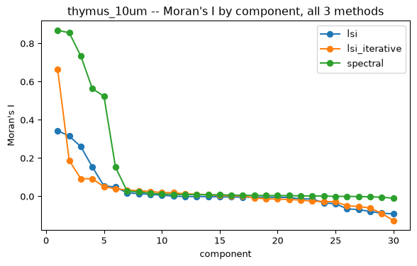
A genuinely informative embedding component should vary smoothly over physical space – nearby tiles should tend to have similar scores – rather than looking like spatial noise. Moran’s I measures exactly that (positive = spatially clustered, ~0 = spatially random). For each method we compute Moran’s I for every component’s per-tile score, then summarize each method by the mean Moran’s I across its components as an overall “spatial informativeness” score.

moran_summary = pd.read_csv("data/moransI_method_summary.csv", index_col=0)
moran_summary

	mean	median	max
method
spectral	0.127455	0.006738	0.867970
lsi_iterative	0.024921	0.003247	0.664328
lsi	0.022765	-0.003491	0.343110

moran_per_component = pd.read_csv("data/moransI_per_component.csv", index_col=0)

fig, ax = plt.subplots(figsize=(7, 4))
for method, group in moran_per_component.groupby("method"):
    ax.plot(group["component"], group["I"], marker="o", label=method)
ax.set_xlabel("component")
ax.set_ylabel("Moran's I")
ax.legend()
ax.set_title("thymus_10um -- Moran's I by component, all 3 methods")
plt.show()

Do spectral and LSI agree?

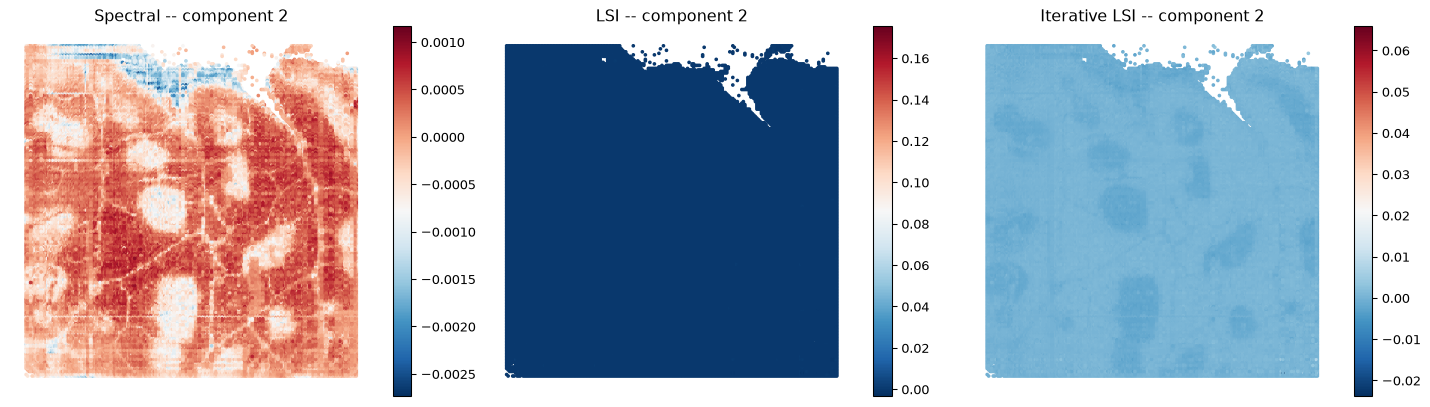
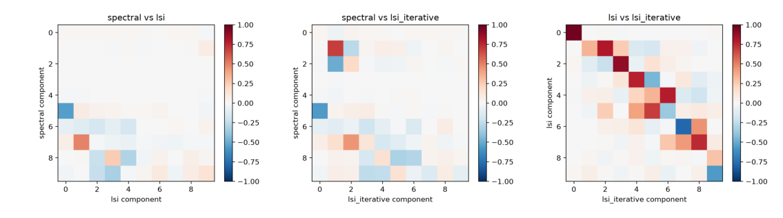
Spectral embedding and LSI/TruncatedSVD arrive at their components through very different math (graph Laplacian eigenvectors vs. TF-IDF-weighted SVD), but if they’re both picking up the same underlying biology, their leading components should still correlate across tiles even though the exact ordering/sign of components isn’t guaranteed to match. We check this directly: spectral’s component 2 vs. LSI’s component 2 (and iterative LSI’s component 2), correlated tile-by-tile.

comp2 = pd.read_csv("data/embedding_correlation_component2.csv")
comp2

	method_a	method_b	comp2_pearson_r	comp2_pearson_p	comp2_spearman_r	comp2_spearman_p	best_matching_component_of_b	best_matching_pearson_r
0	spectral	lsi	0.002464	0.596993	0.046813	8.961811e-24	10	0.072157
1	spectral	lsi_iterative	0.688605	0.000000	0.765236	0.000000e+00	2	0.688605
2	lsi	lsi_iterative	0.342179	0.000000	0.115284	4.855522e-136	3	0.802139

import matplotlib.image as mpimg

img = mpimg.imread("data/embedding_correlation_heatmaps.png")
fig, ax = plt.subplots(figsize=(15, 5))
ax.imshow(img)
ax.axis("off")
plt.show()

Takeaways

Spatial coherence (Moran’s I): spectral wins clearly on this tissue. Mean Moran’s I across components is 0.127 for spectral vs. 0.023-0.025 for both LSI variants – roughly 5x higher. Spectral’s best single component also reaches I=0.87, far above either LSI variant’s ceiling (0.34-0.66). For this thymus dataset, the graph-Laplacian embedding is doing a substantially better job of surfacing spatially organized signal than TF-IDF+SVD does, iterative or not.
Component-2 agreement: spectral and plain LSI do not agree here. Spectral’s component 2 and LSI’s component 2 are essentially uncorrelated (Pearson r=0.002, Spearman r=0.047) – they are not capturing the same axis of variation, despite both nominally being “the second most important direction” in their respective decompositions. That’s a real, dataset-specific result, not a given: agreement between spectral and SVD-family embeddings should be checked per dataset, not assumed from other tissues’ behavior.
Iterative LSI’s payoff: real, but partial. Iterative LSI’s component 2 correlates with spectral’s component 2 much more strongly (r=0.69) than plain LSI does (r=0.002) – the cluster-then-reselect-features step is pulling LSI’s embedding meaningfully closer to what spectral finds. It doesn’t close the Moran’s I gap, though (iterative LSI’s mean Moran’s I, 0.025, is barely above plain LSI’s 0.023) – here, iterative LSI buys better agreement with spectral, not better spatial coherence on its own.

Code for the full pipeline (GEO download through this notebook’s input files) lives in analysis/src/embedding_comparison/thymus_10um/ in the spatial_atac project repo.